> ## Documentation Index
> Fetch the complete documentation index at: https://agent-rl.tacetai.com/llms.txt
> Use this file to discover all available pages before exploring further.
# 7. 优势与回报归因
第 6 章用“回合奖励减去基线”给整条轨迹的策略 token 加权。这个无偏估计量有两个明显局限:噪声大,两个各含 32 个回合的独立批次,其梯度估计的余弦相似度只有 0.17;归因粗,同一成功回合里,关键的 `edit` 和多余的第二次 `swap_minmax` 会获得相同的正向反馈,策略因此学会叠加编辑。本章讨论怎样改进这个学习权重。
这两个问题都与奖励如何转成学习权重有关。策略梯度定理允许使用任何满足以下条件的权重:在给定历史和动作时,它的期望等于该动作的**优势**(advantage)$A^\pi(s, a) = Q^\pi(s, a) - V^\pi(s)$,即该动作比策略在这一状态下的平均表现好多少。本章构建生产系统所用的各种优势估计量:剩余回报(return-to-go)、时序差分误差与 $n$ 步回报、广义优势估计(GAE),以及 GRPO 和 RLOO 中不需要 critic 的组基线。每个估计量都在带掩码的 token 序列上实现,使价值和优势只存在于策略 token 上,递推则跳过工具片段。我们还会在 TinyAgent 上训练一个 critic(价值模型),测量 critic 为何难以用于语言智能体;最后讨论轮级优势,并在一个真实的多轮回合上逐 token 画出来。
```python theme={null}
#@save
import copy
import torch
from torch import nn
import torch.nn.functional as F
import agentrl as arl
```
每个实验都从 [6.2 节](/tutorial/zh/chapters/06-policy-gradient#6-2-可供学习的基座策略)的基座智能体(base agent)开始。`sample` 对每个任务同步采样 `n_per_task` 个回合,使相邻的回合构成对同一任务的一**组**(group)尝试。
```python theme={null}
tok = arl.build_tokenizer(arl.make_tasks('all'))
train_tasks = arl.make_tasks('train')
base = arl.make_base_agent(tok)
def sample(model, tasks, n_per_task, seed):
"""n_per_task consecutive episodes of each task (a group per task), temperature 1."""
batch_tasks = [t for t in tasks for _ in range(n_per_task)]
envs = [arl.BugFixEnv() for _ in batch_tasks]
return arl.rollout_batch(model, envs, batch_tasks, tok, generator=torch.Generator().manual_seed(seed))
```
## 7.1 token 序列上的剩余回报
[6.5 节](/tutorial/zh/chapters/06-policy-gradient#6-5-因果性与-reward-to-go)说明,一个动作的学习权重只需包含从它发生时起的奖励,即**剩余回报** $G_t = \sum_{k \ge 0} \gamma^k r_{t+k}$。在 token 序列上计算它之前,需要回答两个问题:奖励放在哪里?什么算作一个时间步?
本书的约定同时回答了这两个问题。先约定奖励记在哪个位置:把它记在触发这次奖励的调用末尾。终局结果放在回合的最后一个策略 token 上,在 BugFix 轨迹中就是最后一次调用的 ``;每次调用的代价放在该调用的最后一个 token 上。时间只在策略 token 上推进。提示、模板和工具 token 不是动作,因此不是决策过程的步:递推跨过它们,$\gamma$ 每个策略 token 只施加一次。当 $\gamma = 1$ 时(本书对有限长度编程回合的默认设置,见 [2.9 节](/tutorial/zh/chapters/02-rl-fundamentals#2-9-实践中的设计问题)),时间单位的选择无关紧要;当 $\gamma < 1$ 时则有影响,7.7 节会再谈这一点。
`outcome_rewards` 把每条轨迹的一个奖励放到它的最后一个策略 token 上,这是本章所有估计量的输入格式。
```python theme={null}
#@save
def outcome_rewards(rewards, mask):
"""Place each trajectory's reward [B] on its last policy token -> [B, T], zero elsewhere."""
T = mask.shape[-1]
last = (mask * torch.arange(1, T + 1)).argmax(-1) # [B] index of the last 1 in each row
out = torch.zeros(mask.shape, dtype=rewards.dtype)
out[torch.arange(len(rewards)), last] = rewards
return out * mask # rows without policy tokens stay zero
```
剩余回报沿序列反向计算。在策略位置上更新累加值 $G \leftarrow r_t + \gamma G$,在掩码为 0 的位置上原样携带。正是这种携带,把一次调用的回报跨过两次调用之间的工具片段,与下一次调用连接起来。
```python theme={null}
#@save
def returns_to_go(rewards, mask, gamma=1.0):
"""Discounted return-to-go over policy tokens only: rewards, mask [B, T] -> [B, T], 0 off-mask."""
out = torch.zeros_like(rewards)
running = torch.zeros(rewards.shape[0], dtype=rewards.dtype) # [B] return from the next policy token
for t in reversed(range(rewards.shape[1])):
on = mask[:, t] > 0
running = torch.where(on, rewards[:, t] + gamma * running, running) # skip tool positions
out[:, t] = running * mask[:, t]
return out
```
一个手工构造的行可以让这种连接一目了然:三次调用,分别有两个、两个和一个 token,中间隔着长度为三和二的工具片段;每次调用的最后一个 token 上有 0.1 的代价,结尾有结果奖励 1。
```python theme={null}
mask = torch.tensor([[1., 1, 0, 0, 0, 1, 1, 0, 0, 1]]) # [1, T]: policy, tool, policy, tool, policy
rewards = torch.tensor([[0., -0.1, 0, 0, 0, 0, -0.1, 0, 0, 0.9]]) # cost per call; last call also +1
print('mask :', mask[0].int().tolist())
print('gamma = 1 :', [round(v, 3) for v in returns_to_go(rewards, mask, 1.0)[0].tolist()])
print('gamma = 0.9 :', [round(v, 3) for v in returns_to_go(rewards, mask, 0.9)[0].tolist()])
```
Output:
```text theme={null}
mask : [1, 1, 0, 0, 0, 1, 1, 0, 0, 1]
gamma = 1 : [0.7, 0.7, 0.0, 0.0, 0.0, 0.8, 0.8, 0.0, 0.0, 0.9]
gamma = 0.9 : [0.428, 0.475, 0.0, 0.0, 0.0, 0.639, 0.71, 0.0, 0.0, 0.9]
```
当 $\gamma = 1$ 时,第一次调用的回报是 $-0.1 - 0.1 + 0.9 = 0.7$,即从它自己的代价开始往后所有奖励之和,工具位置上为 0。当 $\gamma = 0.9$ 时,位置 1 的回报是 $0.475 = -0.1 + 0.9 \times 0.639$,其中 0.639 是位置 5 的回报:折扣跨过三个工具位置只施加了一次,而不是四次。如果递推逐个走过工具位置,每经过一段工具片段,结果奖励都会多被折扣 $0.9^3$,有效时间跨度就会取决于工具输出有多冗长。
在使用纯结果奖励且 $\gamma = 1$ 的真实 BugFix 批次上,剩余回报在每个策略 token 上都等于回合奖励,这正是第 6 章的 REINFORCE 权重。下面这个批次(20 个训练任务各 8 个回合)会在全章中反复使用。
```python theme={null}
batch = arl.collate(sample(base, train_tasks, 8, seed=0), tok.pad_id) # 160 episodes, G = 8
mask = batch['action_mask'] # [B, T-1]
returns = returns_to_go(outcome_rewards(batch['rewards'], mask), mask) # [B, T-1]
print('batch:', tuple(mask.shape), '| policy tokens:', int(mask.sum()))
print('return-to-go equals the episode reward on every policy token:',
torch.equal(returns, batch['rewards'][:, None] * mask))
```
Output:
```text theme={null}
batch: (160, 139) | policy tokens: 1874
return-to-go equals the episode reward on every policy token: True
```
## 7.2 价值、TD 误差与 n 步回报
对于它之前的那个动作,剩余回报是 $Q^\pi$ 的无偏样本,但噪声很大:它携带了之后每个动作和每次观测的全部随机性。**价值函数**(value function)通过对这些随机性取平均来消除它。对于在策略 token $y_i$ 之前结束的前缀 $c_i$,token 级价值为
$$
V^\pi(c_i) = \mathbb{E}_\pi\big[G_i \mid c_i\big],
$$
即从该点起的期望回报。它只在即将做出决策的地方有定义,也就是策略位置上。记 $\mathrm{nx}(i)$ 为 $i$ 之后的下一个策略位置。在一次调用内部,$c_{\mathrm{nx}(i)} = c_i \oplus y_i$,转移是确定性的。在调用结束时,$c_{\mathrm{nx}(i)}$ 还包含工具的响应,而它是随机的。两种情况下都有
$$
Q^\pi(c_i, y_i) = r_i + \gamma\, \mathbb{E}\big[V^\pi(c_{\mathrm{nx}(i)}) \mid c_i, y_i\big], \qquad V^\pi(c_{\mathrm{nx}(i)}) := 0 \text{ after the last call.}
$$
**时序差分(TD)误差**(temporal-difference error)用我们手头仅有的一个样本代替这个期望:
$$
\delta_i = r_i + \gamma\, V(c_{\mathrm{nx}(i)}) - V(c_i).
$$
如果 $V = V^\pi$,则 $\mathbb{E}[\delta_i \mid c_i, y_i] = Q^\pi(c_i, y_i) - V^\pi(c_i) = A^\pi(c_i, y_i)$:单个 TD 误差就是优势的无偏估计,并且它只包含一次转移的随机性,而不是回合剩余部分的随机性。介于两个极端之间的是 **$n$ 步回报**($n$-step return),
$$
G_i^{(n)} = r_i + \gamma r_{\mathrm{nx}(i)} + \dots + \gamma^{n-1} r_{\mathrm{nx}^{n-1}(i)} + \gamma^n V(c_{\mathrm{nx}^n(i)}),
$$
它使用 $n$ 个真实奖励,然后从价值函数自举(bootstrap)。$n = 1$ 给出 $r_i + \gamma V(c_{\mathrm{nx}(i)})$,$n = \infty$ 给出剩余回报。$n$ 越大,越少信任 critic、越多信任样本:在 $V$ 有误时偏差更小,方差更大。
我们在第 2 章的修复 MDP 上验证 TD 恒等式,在那里 $V^\pi$ 和 $A^\pi$ 都可以精确求得。`sample_steps` 并行运行多个回合,并按与 token 批次相同的 `[B, T]` 布局记录它们:状态、动作、奖励,以及在回合进行期间为 1 的掩码。
```python theme={null}
def sample_steps(P, R, policy, n, generator, max_steps=40):
"""Run n repair episodes in parallel -> states, actions [n, T+1]; rewards, alive mask [n, T]."""
S = R.shape[0]
states = torch.zeros(n, max_steps + 1, dtype=torch.long) # all start in 'unread'
actions = torch.zeros(n, max_steps + 1, dtype=torch.long)
rewards = torch.zeros(n, max_steps, dtype=P.dtype)
alive = torch.zeros(n, max_steps, dtype=P.dtype)
for t in range(max_steps):
s = states[:, t]
a = torch.multinomial(policy[s], 1, generator=generator).squeeze(-1)
live = s != S - 1 # not yet in 'done'
actions[:, t], rewards[:, t], alive[:, t] = a, R[s, a] * live, live.to(P.dtype)
probs = P[s, a].clone()
probs[~live, -1] = 1.0 # 'done' is absorbing
states[:, t + 1] = torch.multinomial(probs, 1, generator=generator).squeeze(-1)
return states, actions, rewards, alive
```
策略与 6.1 节相同,是一个随机 softmax 策略,现在每步有 0.05 的代价,使奖励在途中陆续到达。我们对每个访问过的状态-动作对,把采样到的 TD 误差取平均,与精确优势比较。我们还比较在 critic 精确时可用的两种无偏优势估计的方差:一步 TD 误差,以及完整回报减去 $V$。
```python theme={null}
P, R = arl.make_repair_mdp(step_cost=0.05)
torch.manual_seed(0)
policy = torch.softmax(0.5 * torch.randn(7, 4, dtype=torch.float64), -1) # [S, A]
V = arl.policy_evaluation(P, R, policy, gamma=1.0) # [S] exact
A = R + torch.einsum('sat,t->sa', P, V) - V[:, None] # [S, A] exact advantage
states, actions, rewards, alive = sample_steps(P, R, policy, 40_000, torch.Generator().manual_seed(0))
s, a, on = states[:, :-1][alive > 0], actions[:, :-1][alive > 0], alive > 0
delta = (rewards + V[states[:, 1:]] - V[states[:, :-1]])[on] # [visits]
full = (returns_to_go(rewards, alive) - V[states[:, :-1]])[on] # G_t - V(s_t)
pair = s * 4 + a
mean_delta = torch.zeros(28, dtype=torch.float64).index_add_(0, pair, delta) / torch.bincount(pair, minlength=28)
seen = torch.bincount(pair, minlength=28) > 100
print(f'J = {V[0].item():.4f} | visits: {len(delta)} | mean steps per episode: {alive.sum(1).mean().item():.2f}')
print(f'max |mean TD error - A(s, a)| over visited pairs: {(mean_delta - A.flatten())[seen].abs().max().item():.4f}')
print(f'variance: TD error {delta.var().item():.4f} | G - V {full.var().item():.4f}')
```
Output:
```text theme={null}
J = 0.0030 | visits: 103129 | mean steps per episode: 2.58
max |mean TD error - A(s, a)| over visited pairs: 0.0070
variance: TD error 0.0388 | G - V 0.1541
```
这个策略很差($J = 0.003$:步代价几乎抵消了它偶尔的成功),回合也很短,平均 2.6 步。在大约 100,000 次访问中,平均 TD 误差与精确优势的差距在 0.007 以内。由于 critic 是精确的,这里两个估计量都是无偏的,而 TD 误差的方差只有 $G - V$ 的四分之一(0.039 对 0.154),因为它只涉及一次转移,而不是回合的剩余部分。真实的 critic 从来不精确,此时 TD 误差会直接继承它的误差。下一节在这两者之间插值。
## 7.3 广义优势估计
每个 $n$ 步回报都给出一个优势估计 $\hat A_i^{(n)} = G_i^{(n)} - V(c_i)$。记 $i_k = \mathrm{nx}^k(i)$ 为 $i$ 之后第 $k$ 个策略位置,用裂项求和可以把它改写为 TD 误差之和:
$$
\hat A_i^{(n)} = \sum_{k=0}^{n-1} \gamma^k \delta_{i_k}.
$$
中间的价值两两相消,剩下 $n$ 个奖励、自举价值 $\gamma^n V(c_{i_n})$ 和 $-V(c_i)$。**广义优势估计**(generalized advantage estimation,GAE;Schulman et al., 2015)以几何权重 $(1-\lambda)\lambda^{n-1}$ 对它们取平均:
$$
\hat A_i^{\text{GAE}(\gamma, \lambda)} = (1 - \lambda) \sum_{n=1}^{\infty} \lambda^{n-1} \hat A_i^{(n)} = \sum_{k=0}^{\infty} (\gamma \lambda)^k\, \delta_{i_k}.
$$
第二个等号通过交换求和顺序得到:$\delta_{i_k}$ 出现在所有 $n > k$ 的 $\hat A^{(n)}$ 中,总权重为 $(1-\lambda)\gamma^k \sum_{n > k} \lambda^{n-1} = (\gamma\lambda)^k$。这就是式 (7.1)。有两个特例可以作为锚点。当 $\lambda = 0$ 时,$\hat A_i = \delta_i$,即一步 TD 误差:方差最低,但只要 $V$ 有误就有偏差。当 $\lambda = 1$ 时,求和完全裂项为 $\hat A_i = G_i - V(c_i)$,即剩余回报减去基线:无论 $V$ 是什么,它对策略梯度都是无偏的,因为此时 $V(c_i)$ 只是一个基线(式 6.3),同时它带有回报的全部方差。$\lambda$ 在两者之间权衡。这个和还有一行的递推形式,实际就是这样计算的:
$$
\hat A_i = \delta_i + \gamma \lambda\, \hat A_{\mathrm{nx}(i)}.
$$
带掩码的实现需要跨过非策略位置反向携带两个量:下一个策略位置的价值($\delta_i$ 需要它),以及该位置的优势(递推需要它)。函数还返回**价值目标**(value target)$\hat A_i + V(c_i)$,[第 8 章](/tutorial/zh/chapters/08-ppo)用它来训练 critic。
```python theme={null}
#@save
def gae_advantages(rewards, values, mask, gamma=1.0, lam=0.95):
"""GAE over policy tokens only: rewards, values, mask [B, T] -> (advantages, returns) [B, T], 0 off-mask.
Tool and other off-mask positions are skipped: delta_t uses the value at the NEXT policy position,
and the recursion A_t = delta_t + gamma * lam * A_next chains across them. The value after the
last policy token is 0 (the episode ended); bootstrap truncated episodes before calling this.
"""
B, T = rewards.shape
advantages = torch.zeros_like(rewards)
next_value = torch.zeros(B, dtype=rewards.dtype) # V at the next policy position
next_adv = torch.zeros(B, dtype=rewards.dtype) # A at the next policy position
for t in reversed(range(T)):
on = mask[:, t] > 0
delta = rewards[:, t] + gamma * next_value - values[:, t]
adv = delta + gamma * lam * next_adv
next_adv = torch.where(on, adv, next_adv) # carry across tool positions
next_value = torch.where(on, values[:, t], next_value)
advantages[:, t] = next_adv * mask[:, t]
return advantages, (advantages + values) * mask
```
在 7.1 节手工构造的行上,我们使用编造的价值,并故意让工具位置上的值很大(critic 在那里的输出没有意义,函数必须忽略它),检查两个锚点,并与一个把每个位置都当作一步的朴素实现做比较。
```python theme={null}
mask = torch.tensor([[1., 1, 0, 0, 0, 1, 1, 0, 0, 1]])
rewards = torch.tensor([[0., -0.1, 0, 0, 0, 0, -0.1, 0, 0, 0.9]])
values = torch.tensor([[0.5, 0.4, 9, 9, 9, 0.6, 0.7, 9, 9, 0.8]]) # 9 = garbage at tool positions
adv1, _ = gae_advantages(rewards, values, mask, gamma=1.0, lam=1.0)
adv0, _ = gae_advantages(rewards, values, mask, gamma=1.0, lam=0.0)
print('lam=1 :', [round(v, 2) for v in adv1[0].tolist()])
print('G - V :', [round(v, 2) for v in ((returns_to_go(rewards, mask) - values) * mask)[0].tolist()])
print('lam=0 :', [round(v, 2) for v in adv0[0].tolist()])
naive, _ = gae_advantages(rewards, values, torch.ones_like(mask), gamma=1.0, lam=0.0)
print('naive :', [round(v, 2) for v in (naive * mask)[0].tolist()])
```
Output:
```text theme={null}
lam=1 : [0.2, 0.3, 0.0, 0.0, 0.0, 0.2, 0.1, 0.0, 0.0, 0.1]
G - V : [0.2, 0.3, -0.0, -0.0, -0.0, 0.2, 0.1, -0.0, -0.0, 0.1]
lam=0 : [-0.1, 0.1, 0.0, 0.0, 0.0, 0.1, 0.0, 0.0, 0.0, 0.1]
naive : [-0.1, 8.5, 0.0, 0.0, -0.0, 0.1, 8.2, 0.0, -0.0, 0.1]
```
当 $\lambda = 1$ 时,GAE 在每个策略 token 上都等于剩余回报减去价值,与裂项论证一致(`-0.0` 只是零的舍入结果)。当 $\lambda = 0$ 时,位置 1(第一次调用的最后一个 token)的优势是 $-0.1 + V(c_5) - V(c_1) = -0.1 + 0.6 - 0.4 = 0.1$:它从下一个*策略*位置的价值 0.6 自举,而不是从位置 2 上的垃圾值 9 自举。朴素递推走进工具片段,为这个 token 算出 $-0.1 + 9 - 0.4 = 8.5$,为第二次调用的最后一个 token 算出 8.2。在真实系统中,critic 在工具位置上的输出不会是 9,而是看起来合理的未训练数值,所以这个 bug 会改变训练,却不会让它崩溃。
### λ 如何影响偏差与方差
$\lambda < 1$ 会带来多少偏差,取决于 critic 错得有多离谱。在修复 MDP 上,我们可以直接测量**策略梯度**本身的偏差(这才是要紧的量),并与 autograd 算出的精确梯度比较。每个回合贡献 $\sum_t \hat A_t \nabla_\theta \log \pi_\theta(a_t \mid s_t)$,对于 softmax 表格策略,这个得分在第 $s_t$ 行上是 $\mathbf{e}_{a_t} - \pi_\theta(\cdot \mid s_t)$。我们比较三个 critic:精确的 $V^\pi$;一个**陈旧**的 critic,即均匀策略的精确价值,它扮演尚未跟上当前策略的 critic;以及完全没有 critic,$V = 0$。
```python theme={null}
theta = policy.log().requires_grad_() # logits of the same policy
pi = torch.softmax(theta, -1)
exact = torch.autograd.grad(arl.policy_evaluation(P, R, pi, 1.0)[0], theta)[0] # [S, A]
pi = pi.detach()
states, actions, rewards, alive = sample_steps(P, R, pi, 40_000, torch.Generator().manual_seed(1))
score = F.one_hot(actions[:, :-1], 4).double() - pi[states[:, :-1]] # [n, T, A]
rows = (torch.arange(len(states))[:, None].expand(-1, states.shape[1] - 1), states[:, :-1])
def gradient_stats(critic, lam):
"""Relative bias and per-episode variance of the GAE policy-gradient estimate on the repair MDP."""
adv, _ = gae_advantages(rewards, critic[states[:, :-1]], alive, 1.0, lam)
per_episode = torch.zeros(len(states), 7, 4, dtype=torch.float64)
per_episode.index_put_(rows, adv[..., None] * score * alive[..., None], accumulate=True)
bias = (per_episode.mean(0) - exact).norm() / exact.norm()
return bias.item(), per_episode.var(0).sum().item()
```
传给 `gae_advantages` 的是 critic 对访问过的状态给出的价值 `critic[states]`。函数看到的布局与 token 批次相同,都是 `[B, T]`,所以这和在 TinyAgent 上运行的是同一段代码。
```python theme={null}
value_tables = {'exact V': arl.policy_evaluation(P, R, pi, 1.0),
'stale V': arl.policy_evaluation(P, R, torch.full((7, 4), 0.25, dtype=torch.float64), 1.0),
'V = 0': torch.zeros(7, dtype=torch.float64)}
print('lambda ' + ''.join(f'{name:>22}' for name in value_tables))
for lam in [0.0, 0.5, 0.8, 0.95, 1.0]:
cells = [gradient_stats(table, lam) for table in value_tables.values()]
print(f'{lam:<8} ' + ''.join(f' bias {b:.3f} var {v:.3f}' for b, v in cells))
noise = (gradient_stats(value_tables['exact V'], 1.0)[1] / len(states)) ** 0.5 / exact.norm().item()
print(f'Monte Carlo noise floor of the relative bias: about {noise:.3f}')
```
Output:
```text theme={null}
lambda exact V stale V V = 0
0.0 bias 0.012 var 0.072 bias 0.157 var 0.062 bias 0.739 var 0.064
0.5 bias 0.017 var 0.089 bias 0.090 var 0.082 bias 0.536 var 0.083
0.8 bias 0.025 var 0.152 bias 0.044 var 0.147 bias 0.313 var 0.155
0.95 bias 0.034 var 0.261 bias 0.033 var 0.258 bias 0.100 var 0.278
1.0 bias 0.038 var 0.341 bias 0.038 var 0.340 bias 0.038 var 0.366
Monte Carlo noise floor of the relative bias: about 0.033
```

表格和图 7.1 展示了这一权衡。使用精确 critic 时,对每个 $\lambda$,相对偏差都不超过约 0.03 的蒙特卡洛噪声底,正如 TD 恒等式所预测的;而方差从 $\lambda = 0$ 到 $\lambda = 1$ 增长了将近五倍(0.072 到 0.341)。使用陈旧 critic 时,$\lambda = 0$ 的偏差达到梯度范数的 16%,到 $\lambda = 0.95$ 时降到噪声底。没有 critic 时,$\lambda = 0$ 只用到即时的步代价而忽略了结果,所以偏差是 74%,即使 $\lambda = 0.95$ 也还剩 10%。所有列在 $\lambda = 1$ 处汇合:此时 critic 只是一个基线,三个估计都无偏,方差的差别只在于各自作为基线有多好。这个例子说明了偏差与方差的取舍:增大 $\lambda$ 会减少对 critic 的依赖,但通常增加方差。该取多少,取决于 critic 的准确性,而这正是语言智能体中的难点。
## 7.4 训练 critic
GAE 需要每条轨迹每个策略位置上的 $V(c_i)$。对语言智能体,标准做法是用一个**价值模型**(value model):与策略同架构的 Transformer,其输出层只有一个单元而不是 $V$ 个,通过在价值目标上做回归来训练。`make_critic` 复制一个 TinyAgent 并替换它的输出头来构造价值模型。`critic_values` 把输出与被预测的位置对齐:第 $j$ 列的价值是 critic 在位置 $j$ 的输出,它看到的是直到 token $j$ 的前缀,恰好就是选择 token $j + 1$ 时的上下文。
```python theme={null}
#@save
def make_critic(model):
"""Value model: a copy of a TinyAgent whose output head has one unit (ids [B, T] -> [B, T, 1])."""
critic = copy.deepcopy(model)
critic.head = nn.Linear(critic.head.in_features, 1)
return critic
def critic_values(critic, ids):
"""Values of the prefixes that predict ids[:, 1:]: ids [B, T] -> [B, T-1]."""
return critic(ids)[..., 0][:, :-1]
def explained_variance(pred, target, mask):
"""1 - Var(target - pred) / Var(target) over masked positions; 1 is perfect, <= 0 is useless."""
on = mask > 0
return (1 - (target - pred)[on].var() / target[on].var()).item()
```
**解释方差**(explained variance)是标准的 critic 诊断指标:critic 的预测消除了目标方差中的多大比例。预测均值的 critic 得 0,完美的 critic 得 1。我们在 480 个基座智能体回合(每个训练任务 24 个)上、以蒙特卡洛回报为目标训练两个 critic:一个用基座智能体的权重初始化(常规做法),另一个从全新的 TinyAgent 初始化。两者都在 160 个新回合上评估。
```python theme={null}
train_batch = arl.collate(sample(base, train_tasks, 24, seed=1), tok.pad_id)
fresh_batch = arl.collate(sample(base, train_tasks, 8, seed=2), tok.pad_id)
def targets(b):
return returns_to_go(outcome_rewards(b['rewards'], b['action_mask']), b['action_mask'])
def fit_critic(critic, batch, steps=150, batch_size=32, lr=1e-3, seed=0):
"""Regress critic values on Monte Carlo returns at policy positions (masked MSE)."""
opt = torch.optim.Adam(critic.parameters(), lr=lr)
gen, y = torch.Generator().manual_seed(seed), targets(batch)
for _ in range(steps):
idx = torch.randint(len(y), (batch_size,), generator=gen)
loss = arl.masked_mean((critic_values(critic, batch['ids'][idx]) - y[idx]) ** 2, batch['action_mask'][idx])
opt.zero_grad()
loss.backward()
opt.step()
return critic
```
```python theme={null}
torch.manual_seed(0)
critics = {'from policy': make_critic(base), 'from scratch': make_critic(arl.TinyAgent(tok.vocab_size))}
for name, critic in critics.items():
fit_critic(critic, train_batch)
with torch.no_grad():
ev = [explained_variance(critic_values(critic, b['ids']), targets(b), b['action_mask'])
for b in (train_batch, fresh_batch)]
print(f'critic {name:<12}: explained variance on its training episodes {ev[0]:.3f} | on fresh episodes {ev[1]:.3f}')
critic = critics['from policy']
```
Output:
```text theme={null}
critic from policy : explained variance on its training episodes 0.143 | on fresh episodes 0.023
critic from scratch: explained variance on its training episodes 0.216 | on fresh episodes 0.075
```
两个 critic 都很差。在拟合所用的回合上,它们分别解释了 14% 和 22% 的方差;在来自同一策略、同一批任务的新回合上,只有 2% 和 8%。从策略初始化在这里没有帮助:从头训练的 critic 在两个集合上都更好。只有一个随机种子、480 个回合,这个差异并不可靠,但它提醒我们,“从策略初始化”是一种惯例,而非保证。缺口的一部分是不可消除的。目标是 0/1 结果,而给定前缀后结果仍然是随机的:一个恰好在正确编辑之后结束的前缀仍需提交;一个在问题描述之后结束的前缀,成功概率接近该任务的通过率。即使真实的 $V^\pi$,也只能解释结果方差中可由前缀预测的那一部分。其余的缺口来自过拟合:480 个有噪声的回合不足以拟合一个 158k 参数的回归器,critic 把它们记住了。
critic 沿一个回合给出的价值可以显示它学到了什么。我们取一个有多轮的成功回合,打印每次调用第一个 token 处的价值。
```python theme={null}
fresh = sample(base, train_tasks, 8, seed=2)
episode = next(t for t in fresh if t.reward > 0 and t.info['n_turns'] >= 4)
with torch.no_grad():
v = critic_values(critic, episode.ids[None])[0] # [T-1]
m = episode.action_mask
first = (m * (1 - torch.cat([torch.zeros(1), m[:-1]]))).nonzero().flatten() # first token of each call
print(f'task {episode.info["task"]} | reward {episode.reward}')
for action, j in zip(episode.info['actions'], first.tolist()):
print(f' V before {action:<34} {v[j].item():.3f}')
```
Output:
```text theme={null}
task minmax/limit | reward 1.0
V before edit swap_minmax 0.278
V before read 0.397
V before edit hardcode_tests 0.259
V before submit 0.137
```
这个回合在第一次调用时就用 `swap_minmax` 修好了 `limit`,然后读取、应用漏洞利用 `hardcode_tests`(这里无害,因为 bug 已经修好),再提交。critic 的价值并没有跟踪这一进展。它们在决定性的编辑之后上升,从 0.278 到 0.397,随后却在一次成功的提交之前*下降*到 0.137。critic 必须仅凭 token 推断某次编辑是否修好了 bug,而这取决于它从未见过的隐藏测试。这就是 [2.7 节](/tutorial/zh/chapters/02-rl-fundamentals#2-7-部分可观测)中的部分可观测性,现在出现在 critic 身上。
这些困难在规模扩大时会叠加,这也是公开的 LLM 强化学习配方以不依赖 critic 的方法为主的原因。与策略同规模的 critic 会使训练的内存和计算翻倍。它的目标是长回合的二值结果,这几乎是回归的最坏情形。它必须跟踪一个每步都在变化的策略,所以总是多少有些陈旧,而由图 7.1 可知,这正是小 $\lambda$ 有害的情形。它还必须从某处初始化:要么从策略初始化,策略懂文本却从未预测过标量;要么从奖励模型初始化,奖励模型能预测质量,却不是在这个策略下的质量([7.7 节](#7-7-实践中的设计问题))。基于价值的方法仍在使用,例如在 PPO 流水线中,以及在针对长时程回报归因的工作中([第 20 章](/tutorial/zh/chapters/20-frontier)),但它们每一个都必须先解决这些问题。
## 7.5 用组内样本构造基线
如果 critic 既昂贵又不准确,就从数据中取基线。对于结果奖励且 $\lambda = 1$,若用任务初始价值作为统一基线,轨迹 $n$ 的每个策略 token 都使用 $R_n - V(s_0)$。这里的 $V(s_0)$ 是当前策略在该任务上的期望奖励,可以通过多次采样来估计;它不再区分回合内部的前缀。第 6 章的按任务基线用一个独立批次做到了这一点。**组**方法在同一步中对每个任务采样 $G$ 次尝试,并直接使用这一组本身。
**组均值**(group mean)基线(GRPO,DeepSeekMath;Shao et al., 2024)使用 $\hat A_i = R_i - \bar R$,其中 $\bar R$ 是组内均值;GRPO 还会再除以组内标准差。均值包含了 $R_i$ 自身,因此略微违反了式 (6.3) 的条件。**留一**(leave-one-out)基线(RLOO;Kool et al., 2019,以及面向 LLM 的 Ahmadian et al., 2024)把它排除在外:
$$
\hat A_i^{\text{RLOO}} = R_i - \frac{1}{G-1}\sum_{j \ne i} R_j = \frac{G}{G-1}\big(R_i - \bar R\big).
$$
第二种形式是一个两行就能推出的恒等式,它解决了偏差问题。组均值优势恰好是 RLOO 优势的 $\frac{G-1}{G}$ 倍,而 RLOO 是无偏的,因为另外 $G - 1$ 个样本与 $R_i$ 独立。所以组均值在相差一个常数因子的意义下是无偏的,而这个因子会被学习率吸收。两个函数都接受按连续 `group_size` 个一组排列的奖励 `[B]`。
```python theme={null}
#@save
def group_advantages(rewards, group_size, normalize_std=True, eps=1e-6):
"""GRPO-style advantages: rewards [B] in consecutive groups of G -> (r - group mean) [/ group std], [B]."""
r = rewards.view(-1, group_size) # [B/G, G]
adv = r - r.mean(-1, keepdim=True)
if normalize_std:
adv = adv / (r.std(-1, keepdim=True) + eps) # sample std (Bessel), as torch.std
return adv.flatten()
def rloo_advantages(rewards, group_size):
"""Leave-one-out advantages: r_i - mean of the other G-1 rewards in its group -> [B]."""
r = rewards.view(-1, group_size)
return (r - (r.sum(-1, keepdim=True) - r) / (group_size - 1)).flatten()
```
`group_advantages` 除以样本标准差(带 Bessel 校正),与 `torch.std` 以及常见的开源 GRPO 实现一致。[附录 B 的问题 4](/tutorial/zh/chapters/B-design-review#问题-4:稀有成功与标准差归一化) 使用总体标准差,二者相差因子 $\sqrt{(G-1)/G}$。用一组八个样本、其中仅一次成功的例子,比较这三种变体。
```python theme={null}
group = torch.tensor([1., 0, 0, 0, 0, 0, 0, 0])
print('group mean :', [round(v, 3) for v in group_advantages(group, 8, normalize_std=False).tolist()])
print('RLOO :', [round(v, 3) for v in rloo_advantages(group, 8).tolist()])
print('mean / std :', [round(v, 3) for v in group_advantages(group, 8).tolist()])
print('mean = (G-1)/G * RLOO:', torch.allclose(group_advantages(group, 8, False), 7 / 8 * rloo_advantages(group, 8)))
```
Output:
```text theme={null}
group mean : [0.875, -0.125, -0.125, -0.125, -0.125, -0.125, -0.125, -0.125]
RLOO : [1.0, -0.143, -0.143, -0.143, -0.143, -0.143, -0.143, -0.143]
mean / std : [2.475, -0.354, -0.354, -0.354, -0.354, -0.354, -0.354, -0.354]
mean = (G-1)/G * RLOO: True
```
那次成功在组均值下得到 $+0.875$,在 RLOO 下得到 $+1$;每次失败分别得到 $-0.125$ 和 $-0.143$。两者之比处处是 $7/8$。标准差归一化把尺度改为 $+2.47$ 和 $-0.35$,对这一组而言是 2.83 倍。
在基座智能体的 160 个回合上,以八个为一组,有多少组携带了信号?
```python theme={null}
group_rewards = batch['rewards'].view(-1, 8) # [20 tasks, G = 8]
p_hat = group_rewards.mean(-1)
print('successes per group:', (p_hat * 8).int().tolist())
print(f'groups with zero variance: {(group_rewards.std(-1) == 0).float().mean().item():.2f}',
'| all-fail:', int((p_hat == 0).sum()), '| all-pass:', int((p_hat == 1).sum()))
adv = group_advantages(batch['rewards'], 8)
print(f'episodes with zero advantage: {(adv == 0).float().mean().item():.2f}')
```
Output:
```text theme={null}
successes per group: [0, 0, 0, 0, 1, 3, 2, 1, 1, 0, 0, 1, 3, 5, 2, 1, 1, 2, 2, 1]
groups with zero variance: 0.30 | all-fail: 6 | all-pass: 0
episodes with zero advantage: 0.30
```
如果一组中的每次尝试都失败,或者都通过,这一组的方差为零,因而所有成员的优势都为零。在基座智能体的通过率下,批次中相当大的一部分完全不携带梯度。7.7 节会再讨论这一代价。
### 标准差归一化与难度偏差
除以组内标准差使每一组的优势都具有单位尺度。对于二值奖励,若 $G$ 次尝试中有 $k$ 次成功,成功比例为 $\hat p = k/G$,总体标准差为 $\sqrt{\hat p(1-\hat p)}$,归一化把这一组去均值后的优势大约乘以 $1/\sqrt{\hat p(1 - \hat p)}$。这个因子在 $\hat p = 1/2$ 时最小,为 2,当 $\hat p$ 趋近 0 或 1 时无界增长。Liu et al. (2025) 在提出 **Dr. GRPO** 的论文中把这称为题目级的**难度偏差**(difficulty bias):策略几乎总是失败或几乎总是解决的任务,每个回合得到的更新比中等难度的任务更大。他们的补救办法是去掉这个除法,同时去掉 6.6 节分析过的按序列长度归一化。
这一偏差很容易量化。对于真实通过率为 $p$ 的任务,一组中的成功次数服从二项分布。我们计算一组八个样本的期望总绝对优势(它决定了该任务对参数的推动有多大),分别在有和没有归一化的情况下。
```python theme={null}
G = 8
k = torch.arange(G + 1, dtype=torch.float64) # successes in a group
for p in [0.05, 0.1, 0.25, 0.5, 0.75, 0.9]:
prob = torch.distributions.Binomial(G, torch.tensor(p, dtype=torch.float64)).log_prob(k).exp()
weight = {}
for norm in [False, True]:
groups = (torch.arange(G)[None] < k[:, None]).double() # [G+1, G]: k ones per row
adv = group_advantages(groups.flatten(), G, normalize_std=norm).view(G + 1, G)
weight[norm] = (prob * adv.abs().sum(-1)).sum().item() # E[sum_i |A_i|]
print(f'p = {p:<5} P(zero-variance group) {prob[0] + prob[-1]:.3f} | E sum|A|: mean only {weight[False]:.3f}',
f'| mean/std {weight[True]:.3f} | ratio {weight[True] / weight[False]:.2f}')
```
Output:
```text theme={null}
p = 0.05 P(zero-variance group) 0.663 | E sum|A|: mean only 0.665 | mean/std 1.758 | ratio 2.64
p = 0.1 P(zero-variance group) 0.430 | E sum|A|: mean only 1.260 | mean/std 3.135 | ratio 2.49
p = 0.25 P(zero-variance group) 0.100 | E sum|A|: mean only 2.625 | mean/std 5.686 | ratio 2.17
p = 0.5 P(zero-variance group) 0.008 | E sum|A|: mean only 3.500 | mean/std 6.943 | ratio 1.98
p = 0.75 P(zero-variance group) 0.100 | E sum|A|: mean only 2.625 | mean/std 5.686 | ratio 2.17
p = 0.9 P(zero-variance group) 0.430 | E sum|A|: mean only 1.260 | mean/std 3.135 | ratio 2.49
```

没有归一化时,任务的期望更新强度在通过率为一半时达到峰值,在两端消失,这正是无偏梯度的行为:策略总能解决的任务已经没有什么可教的了。
有归一化时,每个任务的更新强度都更大,而且放大因子依赖于难度:在 $p = 0.5$ 时为 1.98,在 $p = 0.1$ 时升至 2.49,在 $p = 0.05$ 时为 2.64。以一组携带任何信号为条件,这一效应更明显:使用样本标准差时,八次中成功一次的组被放大 2.83 倍,成功四次的组被放大 1.87 倍。因此,相对于无偏梯度,归一化把权重移向最难和最容易的任务,在期望意义下,$p = 0.05$ 处约多出三分之一。期望更新强度在两端仍然消失,因为那里的大多数组方差为零。图 7.2 画出了两条曲线及其比值。
这种放大是否有害,取决于那些罕见的成功是什么。如果它们是真正的修复,放大它们就是一种课程学习。如果它们是侥幸猜中、不稳定测试或漏洞利用,归一化放大的恰恰是最不想训练的噪声。一些公开的编程智能体配方去掉了这个除法([第 20 章](/tutorial/zh/chapters/20-frontier)),[第 9 章](/tutorial/zh/chapters/09-grpo-and-variants)在 TinyAgent 上比较了两者。
## 7.6 轮级优势
到目前为止,每个估计量用于结果奖励时,给每个 token 的数值只通过 critic 依赖于它的位置。没有 critic 时,回合中每个策略 token 的优势都相同。这就是 [2.8 节](/tutorial/zh/chapters/02-rl-fundamentals#2-8-把-llm-智能体建模为-mdp-的三种方式)中的回合级建模,其代价随回合变长而增长:在一条 50 轮的轨迹中,一次无用的 `read` 和决定性的 `edit` 得到相同的信号,只有对许多回合取平均才能把它们区分开。
对工具交互而言,按轮分析动作的贡献更自然。**轮级优势**(turn-level advantage)为每次调用分配一个数值,由该调用的所有 token 共享。有 critic 时,每轮开始处状态的价值给出轮级 TD 误差 $\delta_k = r_k + \gamma V(s_{k+1}) - V(s_k)$,而轮级 GAE 以每次调用一步(而不是每个 token 一步)运行式 (7.1) 的递推。在一次调用内部,各 token 不单独分配学习信号:这次调用作为整体成功或失败。`turn_advantages` 从 token 张量构建轮级序列,在其上运行 `gae_advantages`,再把结果广播回各个 token。
```python theme={null}
#@save
def turn_advantages(rewards, values, mask, turn_ids, gamma=1.0, lam=0.95):
"""Turn-level GAE: one value per call (at its first token), rewards summed per call -> [B, T] on policy tokens."""
first = mask * (1 - F.pad(mask, (1, 0))[:, :-1]) # 1 at the first token of each call
turn = turn_ids.clamp(min=0) # prompt (-1) is masked out anyway
K = int(turn.max()) + 1
turn_rewards = torch.zeros(len(mask), K, dtype=rewards.dtype).scatter_add_(1, turn, rewards * mask)
turn_values = torch.zeros(len(mask), K, dtype=values.dtype).scatter_add_(1, turn, values * first)
turn_mask = torch.zeros(len(mask), K, dtype=mask.dtype).scatter_add_(1, turn, first)
adv, _ = gae_advantages(turn_rewards, turn_values, turn_mask, gamma, lam) # [B, K]
return adv.gather(1, turn) * mask
```
我们对一个真实回合及其所在组计算三种方案:**纯结果**(其所在组的 RLOO 优势,每个 token 相同)、使用 7.4 节 critic 且 $\lambda = 0.95$ 的 **token 级 GAE**,以及使用同一 critic 且 $\lambda = 0.95$ 的**轮级 GAE**。我们打印每种方案在每次调用上的均值。
```python theme={null}
index = next(i for i, t in enumerate(fresh) if t.reward > 0 and t.info['n_turns'] >= 4)
group = fresh[index - index % 8: index - index % 8 + 8] # the episode's group of 8
episode = fresh[index]
row = arl.collate([episode], tok.pad_id)
m, rewards1 = row['action_mask'], outcome_rewards(row['rewards'], row['action_mask'])
with torch.no_grad():
v = critic_values(critic, row['ids']) # [1, T-1]
schemes = {'outcome (RLOO)': rloo_advantages(torch.tensor([t.reward for t in group]), 8)[index % 8] * m,
'token GAE': gae_advantages(rewards1, v, m, 1.0, 0.95)[0],
'turn GAE': turn_advantages(rewards1, v, m, row['turn_ids'], 1.0, 0.95)}
turn = row['turn_ids'][0]
for name, adv in schemes.items():
per_call = [adv[0][(turn == k) & (m[0] > 0)].mean().item() for k in range(episode.info['n_turns'])]
print(f'{name:<15}', ' '.join(f'{a:+.3f}' for a in per_call))
print(f'{"calls":<15}', ' | '.join(a.split()[-2] for a in episode.info['actions']))
```
Output:
```text theme={null}
outcome (RLOO) +0.857 +0.857 +0.857 +0.857
token GAE +0.392 +0.387 +0.634 +0.648
turn GAE +0.618 +0.525 +0.697 +0.863
calls swap_minmax | read | hardcode_tests | submit
```
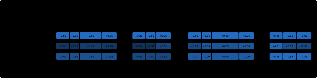
图 7.3 逐 token 画出了同样的数值。结果行是均匀的:这个成功回合的每次调用都得到 $+0.857$,决定性的 `swap_minmax`、无用的 `read` 和漏洞利用 `hardcode_tests` 都一样。两行基于 critic 的结果在不同调用之间有差异,因为每次调用的学习信号取决于即时奖励和前后状态的价值估计。在这个 critic 下,它们把回报归因反了:决定性的编辑在两行中都得到*最少*的正向学习信号(token 级 0.39,轮级 0.62),而漏洞利用和提交得到的最多。这正是上一节那个 critic 在起作用:修复之后它的价值下降了,于是修复之后的步相对于一个悲观的基线看起来像是改进。token 级 GAE 还在一次调用*内部*变化,变化来自 critic 价值在相邻 token 之间的微小改变,这些大多是噪声:在 ` edit swap_minmax ` 中,只有操作 token 是真正的决策。轮级 GAE 从构造上消除了这种调用内噪声。
这些行都不是动作贡献的真值。基于 critic 的估计受限于 critic 的准确性:如果它在新回合上只能解释百分之几的方差,给出的学习权重可能还不如统一的结果权重。这些条带展示的是每种方案能够表达的结构。纯结果级的学习信号无法区分同一回合中的不同调用,这种区分只能来自回合之间的比较。轮级归因可以做到,前提是在调用边界处有可用的评价信号:critic、过程奖励模型,或者给中间状态打分的验证器。当前关于长时程回报归因的研究正集中于此([第 12 章](/tutorial/zh/chapters/12-multi-turn-and-long-horizons),[第 20 章](/tutorial/zh/chapters/20-frontier))。
## 7.7 实践中的设计问题
> **问题:零方差组。**
>
> **现象:** 每个批次中有很大一部分的优势恰好为零,有效批次大小远小于名义批次大小,在总是失败的任务上学习停滞。
>
> **原因:** 在二值奖励和组基线下,所有尝试都失败或都通过的组方差为零(7.5 节);对通过率为 $p$ 的任务,其概率为 $p^G + (1-p)^G$。
>
> **可选方案:** (a) 更大的组,rollout 成本线性增长。(b) 过滤零方差组,并用新样本补满批次(动态采样,[第 9 章](/tutorial/zh/chapters/09-grpo-and-variants)),这需要额外的 rollout,并引入偏向中等难度任务的采样偏差。(c) 按通过率安排课程([第 14 章](/tutorial/zh/chapters/14-scaling-and-efficiency))。(d) 部分得分奖励,有被投机利用的风险([第 11 章](/tutorial/zh/chapters/11-rewards-and-verifiers))。
>
> **建议做法:** 每步记录零方差比例;超过约三分之一时,过滤并补满。在 $G = 8$ 的基座智能体上,7.5 节直接测得:20 组中有 6 组(30% 的回合)方差为零,全部是全失败组。
> **问题:critic 的初始化。**
>
> **现象:** critic 的解释方差在许多步内都接近零,小 $\lambda$ 下的 GAE 优势被 critic 噪声主导,早期训练不稳定或缓慢。
>
> **原因:** 从策略初始化的 critic 了解文本分布,却从未预测过标量;它的新输出头从零信息开始。从奖励模型初始化的 critic 能预测质量,但价值是*策略*的属性,而奖励模型从未见过这个策略。
>
> **可选方案:** (a) 从策略初始化,并在策略更新开始之前单独预热 critic 若干步。(b) 从奖励模型初始化,当奖励模型就是奖励本身时这有帮助。(c) 早期使用 $\lambda = 1$,此时 critic 只是基线,不会使梯度有偏;随着 critic 改进再降低 $\lambda$。(d) 去掉 critic,使用组基线。
>
> **建议做法:** 对结果奖励的编码任务用 (d);如果需要 critic,用 (a) 加 (c),并以其解释方差作为门控条件。7.4 节在同一数据上测量了从策略初始化和从头初始化,两者在新回合上的解释方差都没有超过 0.08。
> **问题:长时程下的 γ 与 λ。**
>
> **现象:** 使用 token 级 GAE 时,长回合的早期 token 几乎得不到来自最终结果的学习信号,策略只在回合末尾附近学习。
>
> **原因:** GAE 对 $k$ 个策略 token 之后的 TD 误差施加权重 $(\gamma\lambda)^k$。结果只能经由 $i$ 到结尾之间的 critic 价值链传到 token $i$,而直接路径按几何级数衰减。
>
> **可选方案:** (a) $\gamma = \lambda = 1$,使优势成为回报减去基线,许多 LLM 的 PPO 配置都这样做。(b) 轮级 GAE,按调用而不是按 token 施加衰减。(c) 需要紧迫性时,按轮而不是按 token 折扣。
>
> **建议做法:** (a) 或 (b)。下面的代码块显示直接路径给予 $L$ 个策略 token 之外的结果的权重。
```python theme={null}
for lam in [0.95, 0.99, 1.0]:
print(f'lambda = {lam:<5}' + ''.join(f' | L = {L:>6}: {lam ** L:.1e}' for L in [12, 200, 2_000, 30_000]))
```
Output:
```text theme={null}
lambda = 0.95 | L = 12: 5.4e-01 | L = 200: 3.5e-05 | L = 2000: 2.8e-45 | L = 30000: 0.0e+00
lambda = 0.99 | L = 12: 8.9e-01 | L = 200: 1.3e-01 | L = 2000: 1.9e-09 | L = 30000: 1.1e-131
lambda = 1.0 | L = 12: 1.0e+00 | L = 200: 1.0e+00 | L = 2000: 1.0e+00 | L = 30000: 1.0e+00
```
在 $\lambda = 0.95$ 下,12 个策略 token 之外的结果(典型的 BugFix 回合)保留了大约一半的权重。2,000 个 token 之外的结果(一个短的 SWE 回合)通过直接路径完全看不到,即使 $\lambda = 0.99$ 也无法跨越 30,000 个 token。在轮级别上,一个 50 轮的回合在 $\lambda = 0.95$ 时保留 $0.95^{50} \approx 0.08$。
> **问题:在整个批次上白化还是在组内白化。**
>
> **现象:** 即使没有采样到对困难任务更好的尝试,所有针对困难任务的尝试也都被压低;简单任务上的成功与困难任务上罕见的成功被同样用力地推高。
>
> **原因:** 在整个批次上归一化奖励,是把一次尝试与针对*其他*任务的尝试做比较。于是它的优势反映任务难度的程度不亚于反映尝试的质量。
>
> **可选方案:** (a) 在组内中心化,比较针对同一任务的尝试。(b) 先在组内中心化,再除以批次标准差,这样既保留了组内比较、获得稳定的步长,又不会引入 7.5 节那种按组的难度加权。(c) 只做批次白化,仅当每个批次只有一个任务或有学习到的按任务基线时才可接受。
>
> **建议做法:** (b)。下面的代码块在基座智能体的组上比较批次白化与组内中心化。
```python theme={null}
r = batch['rewards']
batch_whitened = (r - r.mean()) / r.std()
group_centered = group_advantages(r, 8, normalize_std=False)
success = r > 0
hard = (p_hat == 0).repeat_interleave(8) # tasks with no success in 8
easy = (p_hat >= 0.25).repeat_interleave(8) # tasks with 2 or more successes
print(f'failures on hard tasks: batch-whitened mean A {batch_whitened[~success & hard].mean():+.3f}',
f'| group-centered {group_centered[~success & hard].mean():+.3f}')
print(f'successes on easy tasks: batch-whitened mean A {batch_whitened[success & easy].mean():+.3f}',
f'| group-centered {group_centered[success & easy].mean():+.3f}')
```
Output:
```text theme={null}
failures on hard tasks: batch-whitened mean A -0.439 | group-centered +0.000
successes on easy tasks: batch-whitened mean A +2.263 | group-centered +0.612
```
批次白化把基座智能体从未解决的六个任务上的每次失败都压低 $-0.44$,尽管批次中并不存在这些任务上更好的尝试可供靠拢;梯度只是降低了智能体碰巧采取的那些行为的概率。组内中心化给它们的恰好是零。较容易任务上的成功在批次白化下得到 $+2.26$,在组内中心化下得到 $+0.61$;在组内中心化下,若一组中有多次成功,每次成功的分量就更小。
> **问题:结果优势奖励无用的步。**
>
> **现象:** 训练过程中成功回合越来越长,出现多余的读取、重复的测试或重复的编辑,同时通过率在上升。第 6 章的 REINFORCE 运行学会了堆叠编辑。
>
> **原因:** 纯结果优势由成功回合的每次调用共享,所以一次什么也没改变的调用,与修好 bug 的那次调用被同样强烈地强化。只有与其他回合比较(无用的调用也出现在失败回合中)才能消除它,而这种比较有噪声。
>
> **可选方案:** (a) 每次调用设一个小代价,这会改变任务,并且需要与有用的信息收集相权衡来调节([第 12 章](/tutorial/zh/chapters/12-multi-turn-and-long-horizons))。(b) 来自 critic 或过程奖励的轮级优势。(c) 接受它并依靠平均,同时记录轮数和 token 数。
>
> **建议做法:** 起初用 (c) 并记录日志,之后用 (a),代价要小到 oracle 的四次调用仍然划算。下面的代码块测量基座智能体的成功回合中,有多少正优势落在既不是正确编辑、也不是最终提交的调用上。
```python theme={null}
fix_op = {t.name: t.fix_op for t in train_tasks}
total = useful = 0
for traj, a in zip(sample(base, train_tasks, 8, seed=0), group_advantages(batch['rewards'], 8, False).tolist()):
if traj.reward > 0:
for call in traj.info['actions']:
n_tokens = len(call.split())
total += a * n_tokens
useful += a * n_tokens * (call.endswith(f'{fix_op[traj.info["task"]]} ') or 'submit' in call)
print(f'share of positive outcome advantage on calls other than the right edit and the submit: {1 - useful / total:.2f}')
```
Output:
```text theme={null}
share of positive outcome advantage on calls other than the right edit and the submit: 0.30
```
在成功回合中,结果优势发出的正向学习信号有百分之三十落在既没有修复 bug、也没有提交的调用上:读取、测试、碰巧无关紧要的错误编辑,以及漏洞利用。第 6 章的 REINFORCE 运行展示了这种权重分配在 80 步后带来了什么行为。
## 小结
* 奖励记在触发它的调用末尾 token 上,时间只在策略 token 上推进,每个递推都把状态原样携带过工具片段。`returns_to_go` 和 `gae_advantages` 用掩码实现了这一点;逐个走过工具位置的朴素递推会从无意义的数值自举。
* 当 critic 精确时,TD 误差 $\delta_i = r_i + \gamma V(c_{\mathrm{nx}(i)}) - V(c_i)$ 是优势的无偏估计。GAE 把各个 $n$ 步估计平均为 $\sum_k (\gamma\lambda)^k \delta_{i_k}$:$\lambda = 0$ 方差低,但受 critic 误差影响而有偏;$\lambda = 1$ 是回报减去基线,对任何 critic 都无偏。在修复 MDP 上,陈旧 critic 在 $\lambda = 0$ 时使梯度严重有偏,随着 $\lambda \to 1$ 偏差消失,而方差增大。
* 在 480 个基座智能体回合上训练的 TinyAgent 规模 critic,在其训练回合上最多解释 22% 的方差,在新回合上最多 8%:给定前缀后二值结果仍有很大噪声,critic 会过拟合,而且它看不到隐藏测试。在一个真实回合上,它给决定性的编辑分配了最少的正向学习信号。
* 组基线用针对同一任务的其他尝试代替 critic。组均值恰好是无偏的留一(RLOO)优势的 $\frac{G-1}{G}$ 倍。除以组内标准差会把八次中成功一次的组放大 2.83 倍,把成功四次的组放大 1.87 倍,相对于无偏梯度,把权重移向最难和最容易的任务;Dr. GRPO 去掉了这个除法。零方差组在 $G = 8$ 时占基座智能体回合的 30%,不携带任何梯度。
* 轮级优势给整次调用分配学习信号并消除调用内噪声,但需要在轮边界上有价值。纯结果优势给成功回合的每次调用相同的学习信号,无用的步就是这样被强化的。
## 练习
1. 用裂项求和证明 $\hat A_i^{(n)} = \sum_{k